Project 2
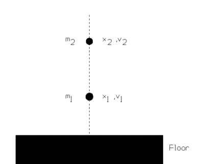
Consider a one-dimensional system that consists of two balls moving along the x-axis in response to gravity, as shown in the figure below:

Collisions between the balls and between the lower ball and the floor are completely elastic, i.e., this is a conservative Hamiltonian system.
Write a program to follow the motion of both balls, where you have to pay special attention to the collision events at which the motion changes abruptly. You can do this either
(a) exactly, i.e., without using finite difference equations if you can look ahead and calculate exact times and positions of the collisions,
or
(b) by using finite difference midpoint method (which actually yields exact, but discretized, solution for motions with constant acceleration):
When the collision with the floor occurs, you should reverse the velocity of the lower ball. On the other hand, when the balls collide with each other, you should use the formula for elastic collisions of two objects (derived in elementary classical mechanics) to find their velocities after the collision.
I) For the three cases: a) m2 = 0.5m1, b) m2 = m1, and c) m2 = 9m1, construct Poincaré sections by plotting v2 against x2 at times when the two balls collide. Take m1 = 1, and use initial conditions x1 = 1, v1 = 0, x2 = 3, and v2 = 0. Which, if any, of these plots indicate that the system is chaotic?
II) Find the position and velocities of the two balls at equal time intervals. Plot x2 against time t for these three cases.
III) Employ the autocorrelation function
which measures self-similarity of a signal with itself in different time intervals (here is the average value of the signal), to analyze the "signal" x2(t) generated by the motion of the second ball. Comment on similarities and differences in the three cases above. In general, we expect autocorellation function to be constant or oscillating for regular motions, while it decays fast to zero (i.e., exponentially) for chaotic motions.
IV) Repeart Poincaré section computation in c) for at least 11 additional sets of initial conditions. For example, you can decrease x2 = 3 in steps of 0.1, while keeping other three variables the same. Plot all 12 Poincaré sections on the same graph and compare with a single Poincaré section you obtained in I) using just one of these 12 sets of initial conditions.
REFERENCES:
1. N. D. Whelan, D. A. Goodings, and J. K. Cannizzo, Phys. Rev. A 42, 742 (1990).
2. Autocorrelation function of discrete and finite data sets.
3. Elementary velocity formulas for elastic collision.